Introductory test for the course Control Systems for Smart Agriculture
Consider the following control system

where $$G(s)=10\frac{1+s}{(1+0.1s)^2}e^{-0.5s}$$.
Design the transfer function \(R (s)\) of the controller in such a way that:
- \(e_\infty=0\) for \(y^o(t)=A\,\text{step}(t)\), where \(A\) is an arbitrary real constant, and \(d(t) = n(t) = 0\);
- a disturbance \(d(t) = D\, \sin (\omega_D t)\), where \(D\) is an arbitrary real constant and \(\omega_D \leq 0.03\, \text{rad/s}\), is attenuated on the output of 100 times;
- a disturbance \(n(t) = N\, \sin (\omega_N t)\), where \(N\) is an arbitrary real constant and \(\omega_N \geq 30 \,\text{rad/s}\), is attenuated on the output of 100 times;
- \(\omega_c \geq 1\, \text{rad/s}\) and \(\varphi_m \geq 50^\circ\) ;
- the controller has at maximum order three.
We start from the steady-state design, considering the gain and type of the controller transfer function.
The steady-state error due to the reference signal, when \(d(t) = n(t) = 0\), is given by
$$e_\infty=\lim_{s\rightarrow 0} s\cfrac{1}{1+L\left(s\right)}\cfrac{A}{s}=\lim_{s\rightarrow 0} \cfrac{A}{1+\cfrac{10\mu_R}{s^{g_R}}}=\lim_{s\rightarrow 0} \cfrac{As^{g_R}}{s^{g_R}+10\mu_R}$$
where \(\mu_R\) and \(g_R\) are the gain and type of the regulator, respectively. In order to have a zero steady-state error we must select \(g_R=1\), independently of the value of \(\mu_R\) and \(A\).
The steady-state design can be thus concluded with
$$R_1\left(s\right)=\frac{1}{s}$$
The transient design, instead, starts with the following loop transfer function
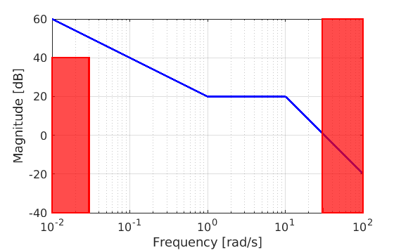
$$L_1\left(s\right)=\frac{10}{s}\cfrac{1+s}{\left(1+0.1s\right)^2}e^{-0.5s}$$
whose magnitude Bode diagram is shown in the following picture.
In order to satisfy the constraints on the attenuation of the disturbances \(d\left(t\right)\) and \(n\left(t\right)\) we must have
$$\frac{1}{\left|1+L\left(j\omega\right)\right|}\leq 0.01\qquad\textrm{for}\qquad\omega\leq 0.03\,\text{rad/s}$$
and
$$\frac{\left|L\left(j\omega\right)\right|}{\left|1+L\left(j\omega\right)\right|}\leq 0.01\qquad\textrm{for}\qquad\omega\geq 30\,\text{rad/s}$$
These two constraints can be approximated as
$$\left|L\left(j\omega\right)\right|_{\text{dB}}\geq 40\,\text{dB}\qquad\textrm{for}\qquad\omega\leq 0.03\,\text{rad/s}$$
and
$$\left|L\left(j\omega\right)\right|_{\text{dB}}\leq -40\,\text{dB}\qquad\textrm{for}\qquad\omega\geq 30\,\text{rad/s}$$
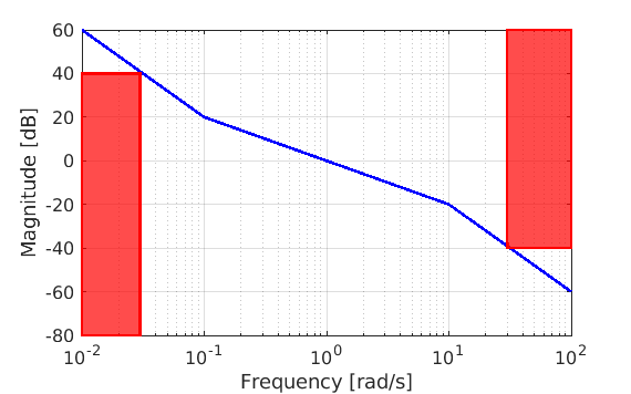
A new loop transfer function \(L\left(s\right)\) can be shaped (see the following picture) having the following expression
$$L\left(s\right)=\frac{10}{s}\cfrac{1+10s}{\left(1+100s\right)\left(1+0.1s\right)}e^{-0.5s}$$
and characterised by \(\omega_c\approx 1\,\text{rad/s}\) and \(\varphi_m\approx 50.5^\circ\), that satisfies the requirements.
The corresponding regulator transfer function is
$$R\left(s\right)=\frac{L\left(s\right)}{G\left(s\right)}=\frac{\left(1+10s\right)\left(1+0.1s\right)}{s\left(1+100s\right)\left(1+s\right)}$$
Consider the following control system
where
$$G(s)=10\frac{1+s}{(1+0.1s)^2}e^{-0.5s}\qquad R(s)=\frac{\left(1+10s\right)\left(1+0.1s\right)}{s\left(1+100s\right)\left(1+s\right)}$$.
Select a sampling time \(T_s\) for the discretisation of the regulator, in such a way that the decrement in phase margin is less or equal to \(3^\circ\), and compute the digital transfer function corresponding to \(R (s)\) using Backward Euler transformation.
Write the pseudo-code to implement the regulator with transfer function \(R (z)\).
The crossover frequency is approximately equal to \(1\,\text{rad/s}\).
We can select the sampling time according to the relation
$$\omega_c\frac{T_s}{2}\frac{180^\circ}{\pi}=3^\circ$$
approximately equal to \(0.1\,\text{s}\).
The digital transfer function \(R\left(z\right)\) can be computed applying the relation
$$s=\frac{z-1}{T_s z}$$
and obtaining
$$R\left(z\right)=\frac{T_s z}{z-1}\frac{\left[\left(T_s+0.1\right)z-0.1\right]\left[\left(T_s+10\right)z-10\right]}{\left[\left(T_s+1\right)z-1\right]\left[\left(T_s+100\right)z-100\right]}=\frac{0.002 z^3-0.003 z^2+0.001 z}{z^3-2.9 z^2+2.8 z-0.9}$$
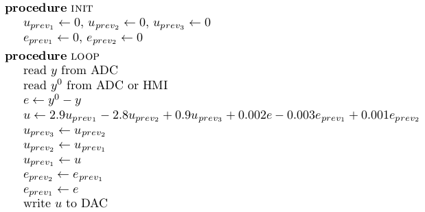
The regulator transfer function can be equivalently rewritten as
$$R\left(z\right)=\frac{U\left(z\right)}{E\left(z\right)}=\frac{0.002-0.003 z^{-1}+0.001 z^{-2}}{1-2.9 z^{-1}+2.8 z^{-2}-0.9 z^{-3}}$$
and translated into a difference equation
$$u\left(k\right)=2.9 u\left(k-1\right)-2.8 u\left(k-2\right)+0.9 u\left(k-3\right)+0.002 e\left(k\right)-0.003 e\left(k-1\right)+0.001 e\left(k-2\right)$$
The control algorithm is shown in the following picture.
Compute the transfer function from \(v_{in}\) to \(v_{out}\) of the circuit shown in the picture below.

Assume \(i_{in}\) is an arbitrary current and \(i_{out}=0\).
Draw the magnitude Bode diagram of the previous transfer function.
Looking at the loop we can write
$$v_{in}=Ri_{in}+v_{out}$$
and the relation between \(i_{in}\) and \(v_{out}\) is given by
$$i_{in}=C\frac{\mathrm{d}v_{out}}{\mathrm{d}t}$$
Merging these two relations, we obtain
$$\frac{v_{in}-v_{out}}{R}=C\frac{\mathrm{d}v_{out}}{\mathrm{d}t}$$
or equivalently
$$v_{in}=v_{out}+RC\frac{\mathrm{d}v_{out}}{\mathrm{d}t}$$
Applying now the Laplace transform to the previous relation we obtain
$$V_{in}\left(s\right)=\left(1+sRC\right) V_{out}\left(s\right)$$
and thus
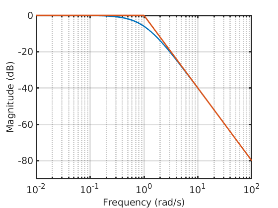
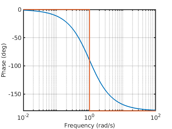
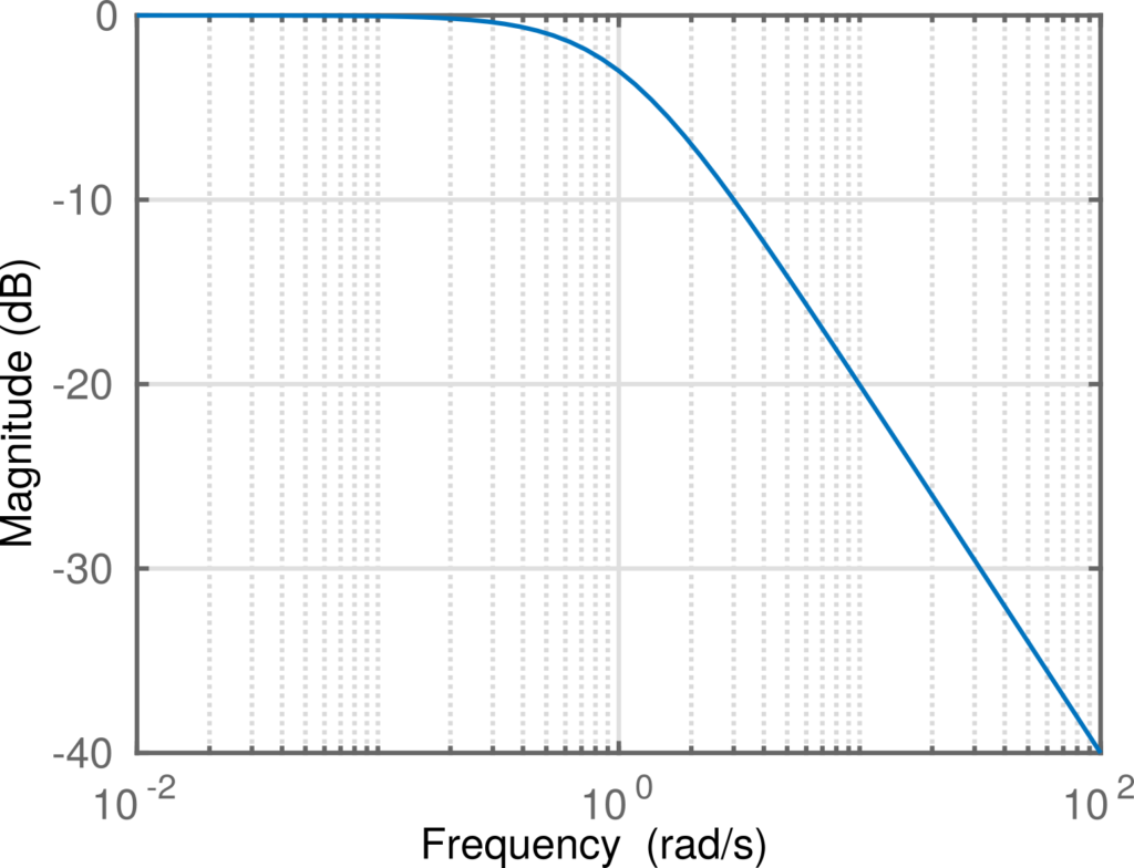
$$G\left(s\right)=\frac{V_{out}\left(s\right)}{V_{in}\left(s\right)}=\frac{1}{1+sRC}$$
The following picture shows the magnitude Bode diagram of \(G\left(s\right)\) for \(RC=1\).
Consider the circuit in the picture below (Wheatstone bridge), and answer to the following questions:

- determine the expression of voltage \(v_m\);
- determine the value \(\bar{R}_G\) of resistor \(R_G\) for which \(v_m=0\) independently of the value of \(V\);
- assuming now resistor \(R_G\) has a resistance \(\bar{R}_G+\Delta R_G\), with \(\Delta R_G\ll\bar{R}_G\), determine the expression of voltage \(v_m\).
Applying Kirchhoff’s rules to the circuit in the picture below

we can write two loop equations and one junction equation
$$\begin{align*}
i &= i_1+i_2\\
V &= \left(R_1+R_3\right) i_1\\
V &= \left(R_2+R_G\right) i_2
\end{align*}$$
From the two last relations we can derive the expressions of \(i_1\) and \(i_2\), as follows
$$i_1=\frac{V}{R_1+R_3}\qquad i_2=\frac{V}{R_2+R_G}$$
and substituting in the first equation
$$i=\left(\frac{1}{R_1+R_3}+\frac{1}{R_2+R_G}\right)V$$
Finally, looking at the loop formed by \(R_1\), \(R_2\) and \(v_m\), we obtain the expression of \(v_m\)
$$v_m=R_2 i_2-R_1 i_1=\left(\frac{R_2}{R_2+R_G}-\frac{R_1}{R_1+R_3}\right)V$$
To determine the value of \(\bar{R}_G\), we have to impose
$$\frac{R_2}{R_2+\bar{R}_G}=\frac{R_1}{R_1+R_3}$$
Solving this relation with respect to \(\bar{R}_G\) we obtain
$$\bar{R}_G=\frac{R_2 R_3}{R_1}$$
Assuming now \(R_G=\bar{R}_G+\Delta R_G\), the expression of \(v_m\) becomes
$$\begin{align*} v_m &=\left(\frac{R_2}{R_2+\bar{R}_G+\Delta R_G}-\frac{R_1}{R_1+R_3}\right)V=\frac{R_2 R_1+R_2 R_3-R_2 R_1-R_2 R_3- R_1\Delta R_G}{\left(R_2+\bar{R}_G+\Delta R_G\right)\left(R_1+R_3\right)}V\\
&=-\frac{ R_1\Delta R_G}{\left(R_2+\bar{R}_G+\Delta R_G\right)\left(R_1+R_3\right)}V \end{align*}$$
If \(\Delta R_G\ll\bar{R}_G\) we can simplify the previous relation as follows
$$v_m=-\frac{ R_1\Delta R_G}{\left(R_2+\frac{R_2 R_3}{R_1}\right)\left(R_1+R_3\right)}V=-\frac{R_1^2}{R_2\left(R_1+R_3\right)^2}\Delta R_G v$$